A step-by-step Guide with photographs and tips on how we perform deep-sky and planetary imaging using a DSLR and CMOS guide camera.

Note: All images in this post are © STAC 2023

Equipment

Before beginning imaging, complete setting up and aligning the equatorial mount as described in Part 1.

Additional equipment we will use here is:

• Guide Camera : ZWO ASI-120mm Mini
• A DSLR as Main Camera to capture the images.
• Laptop to control the camera
• Cables and Batteries for Camera, Laptop, etc
• Optionally, RGB or Light Pollution or other filters

Additionally, install the following software on the laptop :

• Canon EOS Digital / Nikon Camera Control / alternatives to capture photos from the DSLR while connected to the laptop. This way, they can be saved directly to hard disk and the camera can also be programatically triggered to take a sequence of photos without needing a physical intervalometer.
• ASIStudio to control and capture from the ASI Guide Camera. This is the simplest to install, though the popular autoguiding software PHD2 can track objects better. This software will also communicate with the Mount to control the motor based on the guide images.
• Additional drivers (E.g. ASCOM protocol) need to be installed for PHD2. For any software, follow all the instructions from the website and download the necessary libraries/versions for your OS.
• Optionally, Stellarium to identify visible objects and plan what/when to view.
• Siril / Deep Sky Stacker / Autostakkert! / alternatives for stacking, calibrating and post-processing the images.

Note - I have used my personal Canon EOS 550D (unmodified DSLR body) in the photos shown here. Newer models, especially modified for astrophotography, are much better suited. Using a CMOS or CCD camera can be even better still. The types of cameras and pros/cons deserves its own detailed blog post.

Using a DSLR

T-Ring and Adapter

In the image below, the 4 parts from left to right are the Camera body, The T-Ring, Eyepiece adapter (2-part holder and attachment). The T-Ring connects to the camera body in place of the lens. There are different T-Ring models corresponding to different Lens Mounts (e.g. Canon EF/RF, Nikon E/F, etc) and have the appropriate markings and threads to attach them to the body. The eyepiece adapter fits onto the T-Ring using a standardised joint, and into the eyepiece tube of the telescope. Majority of eyepiece adapters have the same specifications, for the standard 1.25” diameter eyepieces (however 2” eyepiece versions also exist, e.g. compatible with STAC’s 8” and 12” Dobsonians).

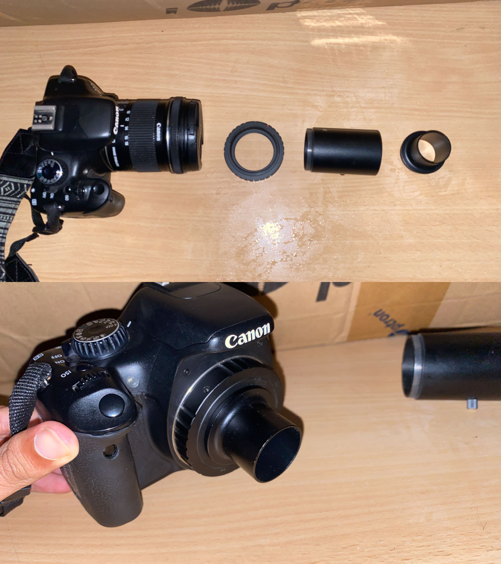
The long tube of the adapter is optional and is meant for holding an eyepiece inside it. It is fixed between the T-Ring and 1.25” telescope adapter to provide a specific magnification / field of view. Otherwise, the camera can be used without an actual eyepiece (connect it to the T-ring without the tube, as shown in the previous image), and the magnification will be fixed, depending on the telescope’s focal length and camera’s sensor size etc. An eyepiece may be good for planetary imaging to provide higher magnification, and also since most planets are quite bright so an extra optical element won’t reduce the quality noticeably. It is unnecessary for most deep-sky targets.

A barlow lens can be attached to the end of the adapter before inserting it in the telescope. Some reasons to use a barlow are:

• Simply to provide more magnification (2x, 3x, etc) if required.
• Depending on the model (physical dimensions) of the Camera body and Telescope, the focal plane may never fall on the sensor as you try focusing the image without any secondary lens. Then a barlow is required extend the focal length so that it can enter the camera.
• To prevent the sensor being exposed (note that with the T-Ring and adapter there is no glass / optical element) to dust and humidity outside. This is not a problem with our Cassegrain telescope, but in a Newtonian/Dobsonian which has an open tube, air can flow all the way in.

Note that DSLR bodies are already relatively heavy compared to the OTA, and by using a barlow or the eyepiece adapter tube, it extends further away from the center and can add a lot of extra torque. Check the balance of the mount as described in Part 1 and re-balance on any axes if necessary.

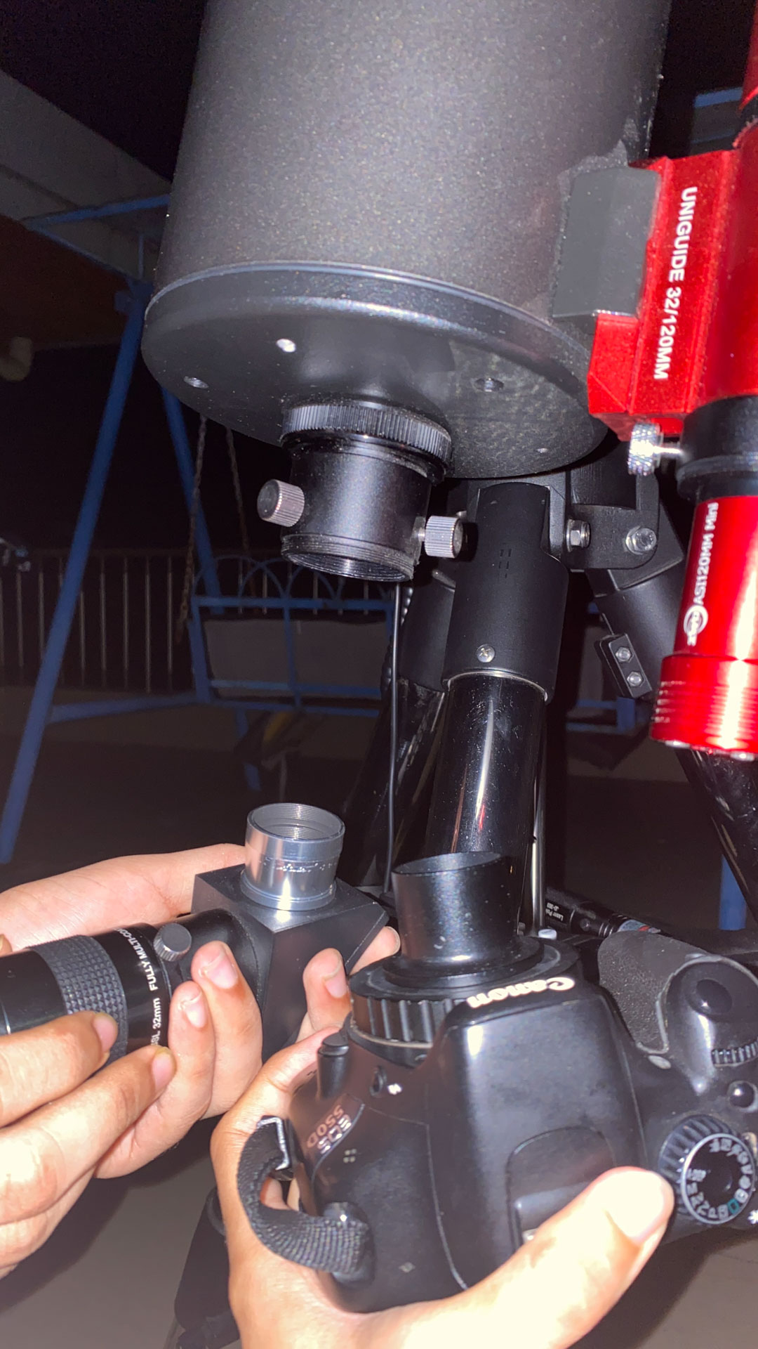
Insert the adapter directly into the telescope, by removing the eyepiece diagonal, which is unnecessary and can also become a weak point where the camera can fall off due to the weight applied sideways while turning as the telescope rotates (and will also cause more Third axis imbalance).

Capture Schedule

Once you have connected the camera to the telescope, switch it on and slew the telescope to a bright object (E.g. Jupiter, The Moon etc which have surface details) to set the focus using the eyepiece focuser. For more precision, use the camera’s live view with digital zoom or connect it to a laptop as described below and zoom into the image. Don’t estimate the focus based on nebulae/galaxies which naturally appear slightly blurry. If perfect focus doesn’t occur at any distance, change/add the barlow lens.

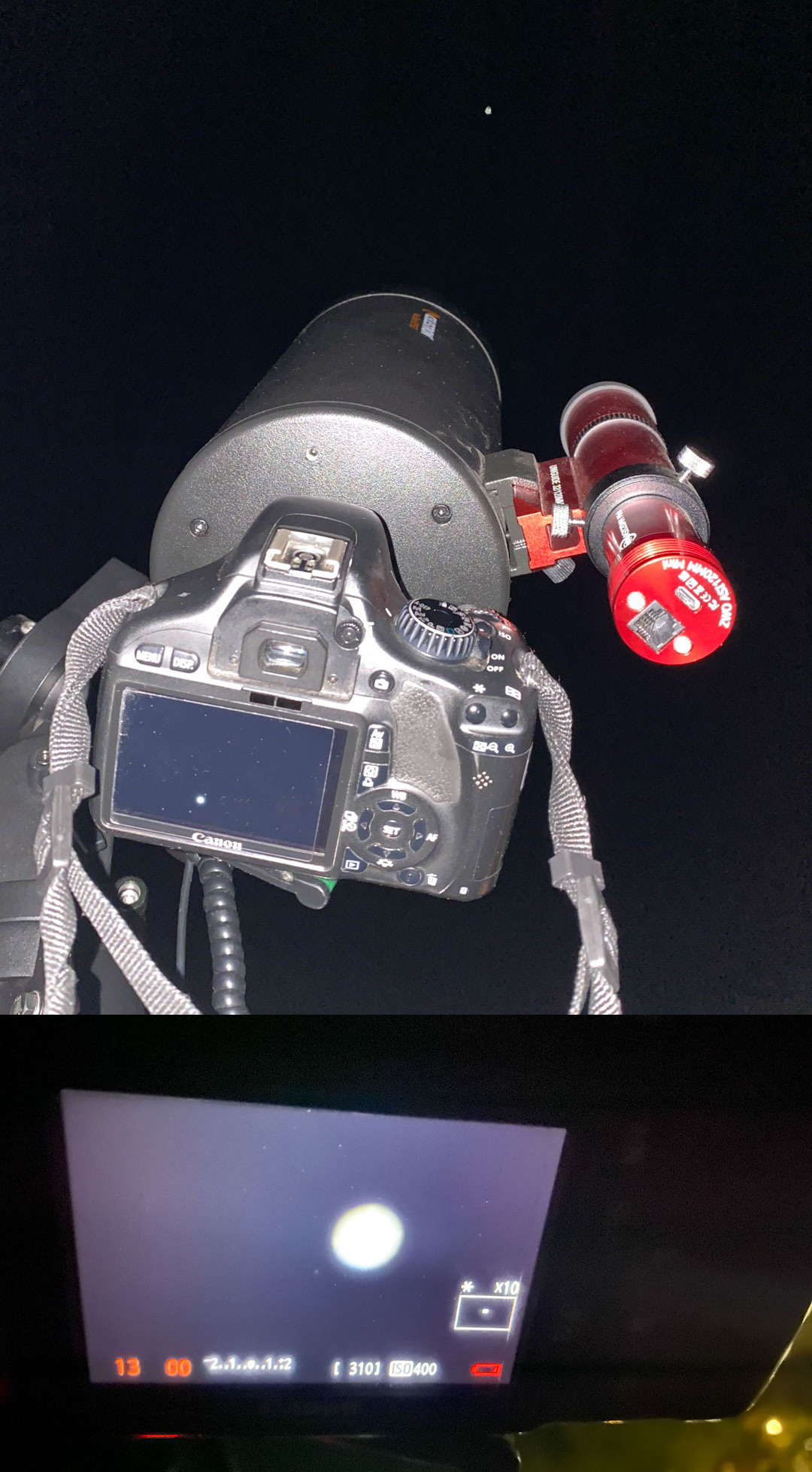
It is possible to image directly from the camera by manually pressing the shutter button. However it may increase small shake and alignment errors each frame, and there are a very large number of frames that typically need to be taken (as described in Calibration below) and timed for specific durations, hence using an intervalometer is preferable. Physical intervalometers exist that connect to the camera like a wired remote control, however we use a laptop since the software on it is typically free of cost, the larger screen is useful for inspecting image quality, and it is anyway needed for autoguiding.

Connect the camera to the laptop using an appropriate data-cable (often USB Mini-B / Micro to USB Type A/C), and start the camera’s native software (e.g. Canon EOS Digital, or Nikon Camera Control, or alternatives) for remote shooting.

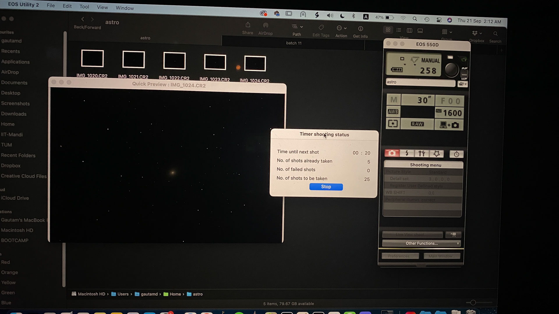
Important: Set the camera to capture in RAW format (e.g. Canon CR2 or Nikon NEF etc) so that all the original data from the sensor is stored without compression.

Exposure settings

We operate the camera usually on fully manual BULB mode for exposures > 1 minute, and set the ISO and exposure time as required. The camera’s focal length is that of the telescope (plus barlow lenses etc that modify the focal length, if used), and will not change since a regular lens isn’t connected. Setting the appropriate ISO and Exposure time depends on the target object. Generally, to reduce noise, try to minimise the ISO and maximise exposure time per frame, while retaining visible clarity and avoiding trailing.

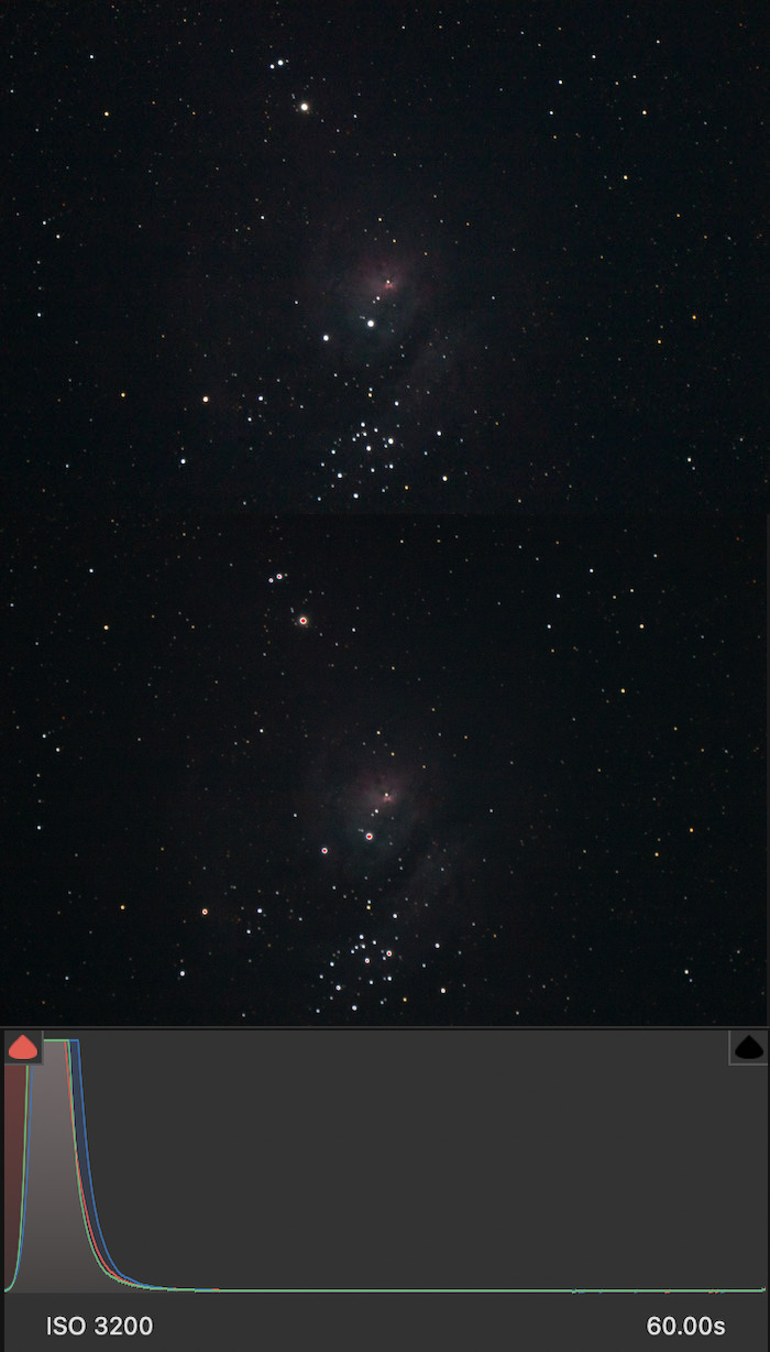
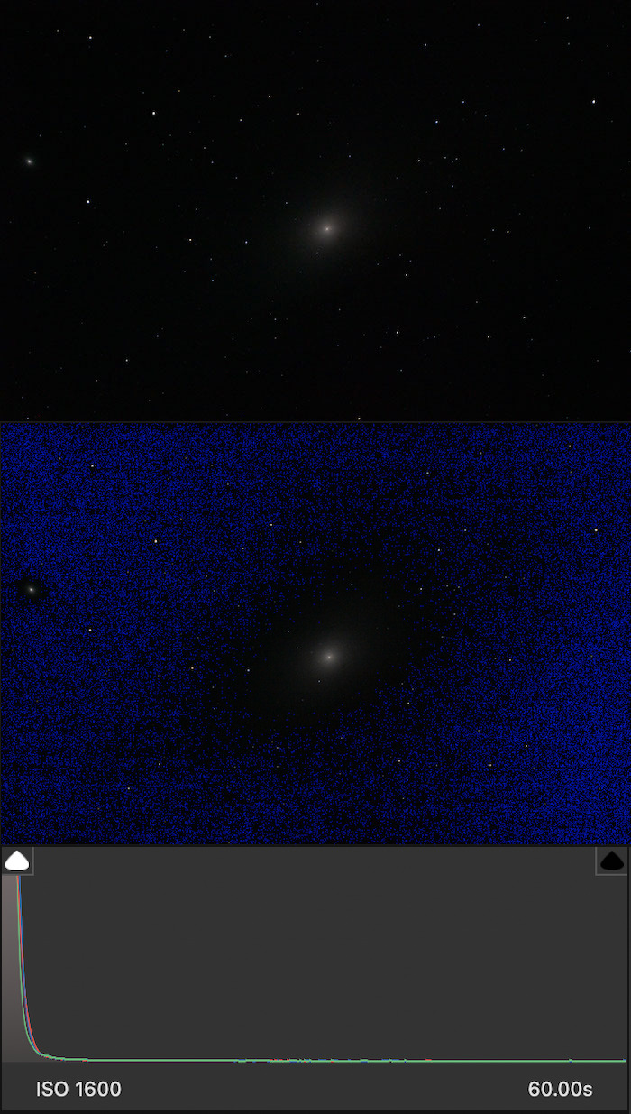
For a good exposure, it’s okay even if very few details are directly visible in the RAW frame, but it is important to check the percentage of clipped pixel values from the image histogram. For example, in the images below, the original raw frame is displayed on top, followed by the preview in Adobe Camera Raw which highlights clipped black pixels in blue and clipped white pixels in red, and the histogram at the bottom. The image of M8 on the left is good, hardly any pixels are clipped to a value of 0, while the image of M31 on the right is underexposed, many are clipped and not just in corners but in most of the area. The histograms of both appear clumped towards the left, since majority of the background is dark, but by zooming in it is clear that in M8 the left/rising edge of the distribution curve is visible while for M31 it is clipped by the y-axis.

If long-exposure shots (e.g. 2-5 minutes or more per frame) are necessary to capture the target, check the quality and trailing effects in a test image. Even if the mount’s balancing and alignment is excellent, small errors can add up while tracking and form trails over several minutes. Then, you can use an auto-guider to prevent trails.

Filters

After setting up the camera, capture a large set of photos (atleast 10-50) that will be stacked together. The importance of stacking is explained in last section (essentially, it improves the signal-to-noise ratio). In case you plan to use filters for imaging, take several shots to stack that many more times, for each filter.

Attach a filter onto the end of the T-adapter (or barlow) before inserting it into the telescope, as with a regular eyepiece. STAC currently has only 2 filters - the neutral density filter for moon and bright planets, and a light pollution filter.

With DSLRs that have RGB sensors, using colour filters is not required. To capture colour images with a monochromatic CCD or CMOS camera (useful for advanced photometric analysis), we will need colour filters such as narrowband (Hα + Oii + Siii is a popular combination of emission wavelengths for deep sky targets) or broadband (LRGB). Dedicated astrophotography software used with such cameras may also allow setting schedules to capture multiple series of raw frames with pre-specified settings, for each filter used.

Autoguiding

Connecting the Guide Cam

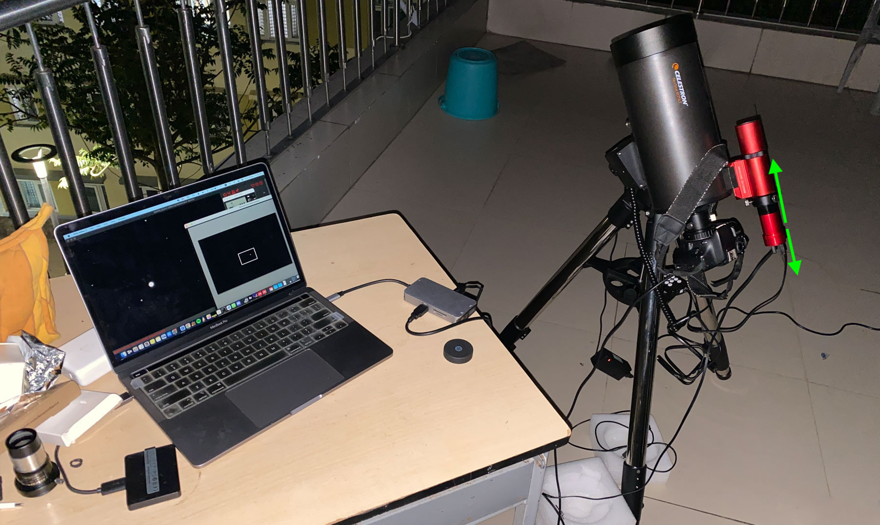
Remove the front cap of the ASI 120mm Mini Camera, insert the camera into the finder scope of the telescope, and fix it securely. Note that the sensor is exposed so make sure not to allow dust or humidity etc to damage it by leaving the cap open for long. There are 2 cables that need to be connected:

• A USB-C to USB-A cable to connect the output feed from the type-C port on the back of the camera to the laptop.
• A non-coiled RJ45 (ethernet-type) cable from the laptop to the GUIDE port on the mount, to send the tracking control signals.

The camera receives power through the first cable itself, so ensure that the laptop remains powered on. To set the focus, we need to view the live feed from the camera via the controller software.

ASI Studio

From the ASI Studio suite, open the ASICap Planetary Imaging app. In the panel on the right, find the list of detected cameras, select ASI 120mm Mini and click on Connect to use the camera. If it doesn’t appear, check the cable connection from the camera to laptop and that the software was installed correctly. Then you will start seeing a live feed from the camera in the main window.

If the focus is incorrect, you may not be able to see any stars in the feed. To set focus, loosen the screws of the finder scope that are holding the camera and slide it further in or out of the scope - the blurry disks of some bright stars should appear and eventually sharpen at the correct length. Tighten the screws again to fix the camera in place. It might help to slew the telescope to a bright star or planet to set the focus. Also set the Guide cam’s Exposure time (usually > 500ms unless a bright star or planet is in the frame) and Gain (analogous to ISO in DSLRs) from the Exposure controls in the right side panel, in case the stars appear very faint.

In case the finder scope wasn’t aligned exactly parallel to the main telescope, you may not see the same target object in the center of the image. The software doesn’t have to track the exact same target being photographed with the main camera to send corrections to the mount motor, nearby stars can also suffice as long as the image is in good focus.

Slew the telescope back to the main target to photograph, check the alignment in the DSLR, and then start auto-guiding by clicking on the “play” triangle icon above the guide cam feed in the ASICap window. The software detects all visible stars in the field and automatically selects an appropriate one as a reference position to check the deviation of the tracking mount. When tracking is active, the reference star’s original position will be circled in the camera feed, and the play button changes to a cross, with 4 arrows. The arrows flash to indicate corrected direction, and you can press the cross to stop auto-guiding. You should now be able to capture longer frames from the DSLR without visible trailing.

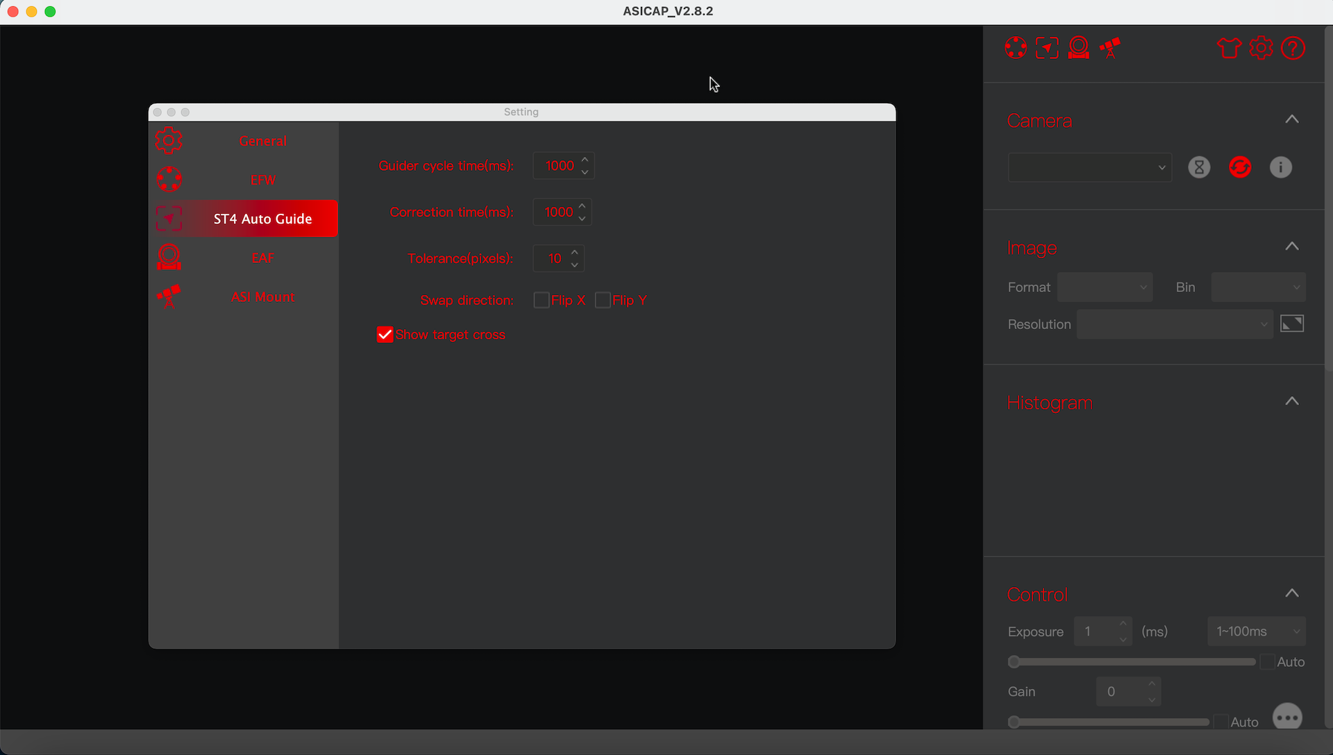
From the ST4 Auto Guide Settings icon at the top of the right panel, you can set the Guider cycle time (interval after which reference star’s deviation will be checked), Correction time (interval after which the mount’s tracking will be adjusted) and Tolerance (threshold to determine whether the reference star’s position has deviated).

Note:

• In case it displays an error about being unable to find stars to track, verify that atleast 4-5 stars are clearly visible in the feed. Adjust the gain/exposure or focus or very slightly modify the region that the camera points at to include more stars, and try starting the autoguider again.
• In some instances in my experience, the guiding stops functioning accurately after 8-10 minutes and allows the star position to drift. In case the reference star in ASICap is far outside its circled original position, stop and re-start the autoguiding.

Calibration Frames

The regular RAW images of the target are known as Light frames. But they contain multiple sources of noise and other errors, besides the random noise reduced by stacking, which get exaggerated during post-processing and histogram stretching, and capturing these calibration frames are important to minimise noise and error from systematic sources.

Note: These also need to be stacked to create a “master” calibration frame of each type, so take atleast 8-10 of each type.

Darks

These frames must be captured using the same settings as lights - same ISO/Gain, same Exposure time, and also while the sensor is at the same temperature. Theoretically, darks taken at another time can be reused as long as these 3 parameters were the same. Else, maintaining their values, take a series of frames by covering the lid of the telescope tube so that no light enters. They reveal:

• Thermal sensor noise that is inherently present even when there is no light/signal from the sky. It is exaggerated by ISO/Gain, collects over the exposure time, and originates at a rate depending on the sensor temperature.
• Hot pixels, which are defective pixels in the sensor that are always on (maybe in just some of the R/G/B channels), appearing as individual bright coloured/white dots.

The image below shows what a single raw dark frame looks like (left), and the exaggerated/stretched noise patterns in the stacked master dark (right).

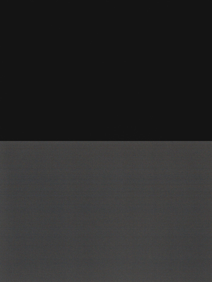
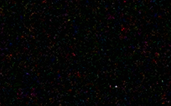
To illustrate the effect of sensor temperature on noise, below are 2 zoomed-in sections of dark frames with the same camera, ISO and exposure time. The one on the left is taken from Mandi campus at an ambient temperature of 13°C, and the one on the right from Hanle at -11°C. The brightest pixels in either are hot pixels.

Flats

These frames are captured by allowing un-textured, uniform light to enter the telescope and clicking an image that is moderately exposed. This reveals:

• Vignette that is caused by the telescope’s optics
• Shadows of dust and scratches on the lenses/mirrors/sensor etc

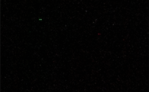
For even illumination, open the telescope lid and point it at an area of clear sky in daylight/twilight the morning after the observing session, or fill the laptop screen with a plain white image and place it onto the aperture to cover it without any gaps. Make sure that the camera’s focus hasn’t shifted so that the shadows aren’t blurred. While clicking the frames, use any ISO/Gain and Exposure time so that the colour range in the image is around 50% grey (on DSLRs you can set a moderate ISO and use Shutter priority (Tv) mode to automatically capture just long enough to moderately expose the image). Slight colour tint is okay, but the entire histogram curve should be around 50% (no white/black). A single raw flat frame (left) and exaggerated/stretched shadows and effects (right) from the stacked master are shown below :

It is important to take flats during the same session and with the same focus, so that the patterns of dust and scratches that were present that night are recorded - these change when the equipment is shifted so flats shouldn’t be reused.

Some image processing guides also use Dark Flats, with the same settings as these flat frames but by covering the telescope lid so that the noise present in flat frames is revealed & can be subtracted from the regular flats.

Biases

Bias frames are captured almost identically to darks (same ISO, without light), but the exposure time is set to the minimum possible value (usually 1/4000 or 1/8000 in DSLRs). This reveals the “sensor read noise” which is due to errors in just saving the image from the sensor when pixels should be almost 100% black. A single raw bias frame (left) and exaggerated/stretched noise (right) from the stacked master are shown below :

Biases can be reused for any other photographs taken with the same camera and ISO/Gain, so it isn’t necessary to capture them next time if a master bias exists. In case the read noise is very low, biases can also be skipped and are not as important as darks and flats.

Post-Processing

The steps for stacking and editing the photos are as important as all the work so far in capturing, to bring out details from the raw frames. This section only has a very brief summary of the procedure and tools used, since there are many different apps and possibilities, and detailed tutorials for each software.

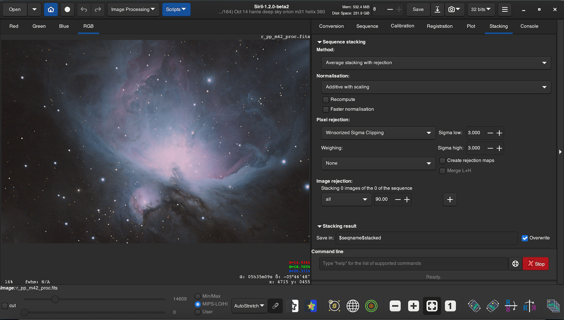
Siril is a good starting point since it has a beginner-friendly UI, it’s also general-purpose (performs calibration, stacking, and some post-processing, also for both planetary and deep sky images), is open source and free of cost, is available for all OSes (Windows/Mac/Linux), and can get advanced when required with plugins and scripting etc, to name a few advantages.

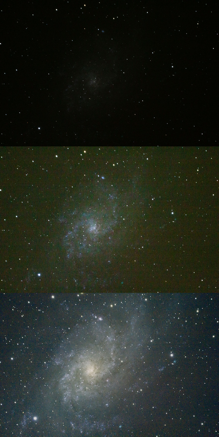
To illustrate the importance of stacking and calibration, below is a single RAW frame of M33, the same raw frame with basic histogram transformations applied to bring out more detail, and then the image from a stack of 28 calibrated frames after complete post processing in Siril.

Stacking

Repeat the procedure outlined below for each set of frames to stack (biases, darks, flats, lights+filters). Stack the calibration frames first, then the lights.

1. Start Siril and Open the Directory containing all the raw frames.
2. For a set of images to stack, create a FITS sequence from RAW filetypes, by adding images into the Conversion panel on the right. To view and edit RGB images in colour, check the Debayer option.
3. The first frame of the sequence is displayed in the window - to highlight details change the viewing mode to “Autostretch” from “Linear” in the bottom panel.
4. When stacking the calibration frames (darks/flats/biases/etc), skip directly to step 8 for the actual stacking.
5. Select the master darks/flats/biases that you earlier stacked, in the Calibration panel, and calibrate the current sequence to create a new “pre-processed” (pp-) sequence. Notice the difference in detail from the raw light frames after calibration. In essence, the operation performed here is Calibrated = (Light - Dark) / (Flat - Bias) for each pixel.
   Note: In case the dark frames you took were at the wrong setting and contain more amplified noise then they should, Siril will display the errors for negative pixel count after dark subtraction.
6. In the Registration panel, align any offset/shake between the pre-processed frames. This automatically detects stars using the algorithm selected (E.g. Global star alignment, 1-2-3 stars, etc) and transforms each image so that all stars are features exactly overlap before stacking, and saves the new version in a “registered pre-processed” (r-pp-) sequence.
7. The Plot panel displays a metric (by default FWHM) of image quality of each registered image. Shaken and blurry images will have a larger FWHM value, and should be discarded before stacking, to preserve detail.
8. Now stack the sequence from the Stacking panel. For calibration frames, use only median or average+rejection stacking. For darks/biases, never apply normalization and for flats, apply multiplicative mormalization. For the registered pre-processed light frames, use any appropriate stacking algorithm (often average+rejection) and normalization. The output is a single FITS image - which is the master frame for calibration, or the output to pre-process in case of light frames.
9. Observe the edges of the stacked frame - it may be more noisy around the edges since frames were translated/scaled/rotated during registration and so data from only some images in the sequence overlaps there. Crop all the edges with a wide enough margin to retain only the main part of the stacked image. Save the FITS file for post-processing/enhancement.

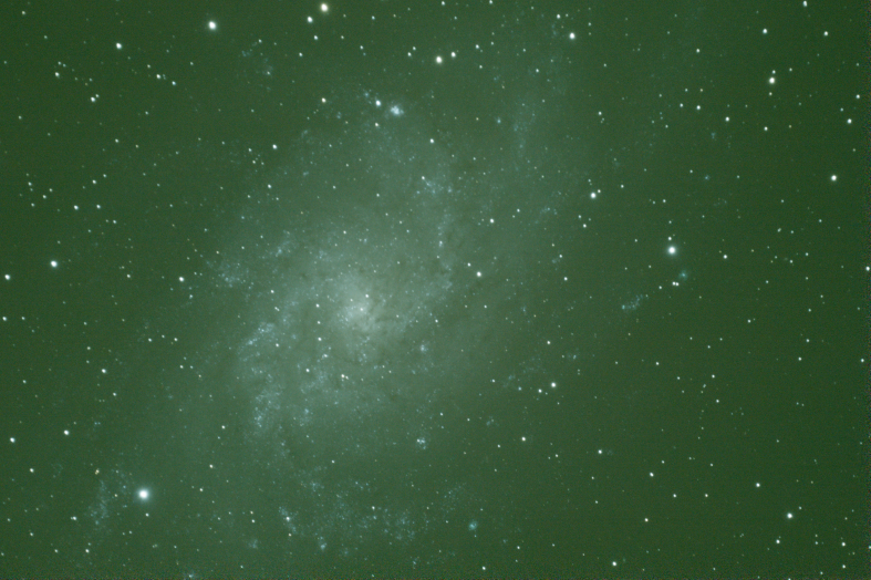
It is natural for colour images taken with a DSLR to appear very greenish by now (due to the RGGB bayer pattern in sensors). This will be corrected in the next step. In case you took images with a monochrome camera and filters, they will still be separate greyscale frames and can be color-composited in the next stage.

Enhancement

In this phase, multiple operations are possible to bring out detail in the image that was calibrated and had reduced noise after stacking. This is a glossary of some of the operations that can be performed (tools are available in Siril from the Image processing dropdown at the top of the window). Important - Change the viewing mode back to “Linear” from “Autostretch” in the bottom row of Siril before beginning pre-processing, to view the true distrbution.

• Histogram Transformation: Modifies exposure / brightness, contrast, highlights, etc like the “Curves” tool in Adobe Photoshop or Lightroom. The histogram can undergo a simple Asinh function stretch, Hyperbolic stretch, or generalised transform. You would typically need to use this first to increase the pixel values from near zero, so that it resembles the autostretched view.
• Remove Green Noise: One click operation to remove the excessive green intensity and obtain a greyish average colour.
• Color calibration: Adjust color balance manually, or using the Photometric tool, to automatic values by specifying the object in the image so that Siril computes the photometric data and looks up the right color saturation values from an online database.
• Deconvolution: A technique to increase sharpness of the image by computing the PSF (point spread function) of “how blurry or spread out” point sources of light are in the image, and using it to increase the contrast at edges. Richardson-Lucy algorithm is used for stars, while Wiener and Split-Bregman algorithms are for sharpening details on Planetary disks (not deep sky images).
• Wavelet Transform: Computes the image features as a combination of N levels of detail in increasing frequency (similar to Fourier Transform), and allows you to change the amplitude of each, affecting the brightness and sharpness of various features in the image.
• Median Filter and Bayes Denoising: Noise reduction algorithms
• Background Extraction: Corrects vignette and non-uniform gradients in the background by sampling the image across a grid, except for points that lie on a “foreground” target object, computing the variation in brightness as a polynomial function, and making it even/flat.
• RGB Compositing: Used to merge stacked and calibrated frames for different channels into a single RGB image.

Apply any of these operations and more in the order as required to improve the quality of the final image.

Further Reading

The steps outlined in this Post-processing section are only a very brief summary of the possible workflow. Some useful tutorials and documentation for Siril (in detail) are:

• https://siril.org/tutorials/
• https://free-astro.org/index.php/Siril:Tutorial_preprocessing
• https://siril.readthedocs.io/en/latest/Processing.html

Some other popular apps include:

• Deep Sky Stacker for generic stacking and calibration.
• AutoStakkert! for stacking planetary images specifically.
• Pixinsight for post processing and Enhancement